LM Descent to the Moon - Part 5 - Powered Landing Maneuver (1964)

(LEM Powered Landing Maneuver, 1964)

[This is a partial reprint of a 1964 technical paper from MIT/NASA, which explains the mathematics behind the 1960's lunar landings. See /1/ for details. LM was called LEM (Lunar Excursion Module) those days and the first landing was to be done summer 1969, 5 years after this paper was written. The strength of this algorithm is that it is real time adaptive to the variations of the parameters from different sources (and also errors). This algorithm was called "E Guidance" due to the E matrix used in it. The basic LM descent guidance logic was defined by an acceleration command which was a quadratic function of time and was, therefore, later termed "Quadratic Guidance". ]

Figure 0. Look angle "lambda" is relative to the thrust axis

POWERED LANDING MANEUVER /1/

1 General Description

"The powered part of the landing maneuver starts at the LEM engine ignition point of the descent orbit and terminates at lunar surface touchdown. The LEM powered landing maneuver has been divided into the three major phases illustrated in Fig. 1.

Figure 1. Lunar landing maneuver phases

1. The first phase is inertially guided and is the longest with respect to time and ground range. The primary GN (Guidance and Navigation) system objective of the first phase, is to achieve a position and velocity condition for the start of the second phase which will allow a near constant vehicle attitude and landing site visibility as the LEM approaches the surface. The scale of Fig. 1 is exaggerated in that the landing site is below the lunar horizon relative to the engine ignition point and does not come within view until the LEM is about 125 n.m. away. For the optimum dV type landing trajectory, the landing site is not visible with the current LEM window configuration until hover conditions have been achieved. For this reason the landing trajectory is shaped such that a vehicle attitude that permits landing site surveillance is achieved during some phase of the maneuver.
2. The desired vehicle attitude during the second phase is such that the astronauts can visibly check the landing area through the LEM windows. The second phase is guided at approximately half-maximum throttle setting in order to lengthen the maneuver time to about two minutes for visual and landing radar updating of the inertial guidance units. The terminal objective of the second phase is to achieve hover or zero velocity conditions over the desired landing site at some pre-designated altitude.
3. The third phase is the let-down and surface landing from the hover condition.

2 Lunar Landing Steering Equations

2.1 General Comments

The lunar landing steering equations are a direct, exact solution to the equations of motion. They express the solution thrust vector as an explicit function of the current position and velocity vectors and the desired position and velocity vectors. Figure 2 is a simple block representation of the equations.

Figure 2. Block diagram of Lunar landing equations.

In mathematical parlance, the lunar landing equations are a solution to a two-point boundary-value problem. The first point is the current state (point in state space); the second point is the desired state. Because the equations express the components of the solution thrust acceleration vector as explicit algebraic functions of literal symbols for the current and desired states, any meaningful and physically reasonable numerical values may be substituted for the literal symbols. This flexibility of the landing equations is quite significant because at least two, and probably more than two, different boundary-value problems will be posed to the guidance system during the landing maneuver.

If the first two phases of the landing maneuver (from engine ignition to the hover point) were accomplished in one powered maneuver, the attitude orientation of the vehicle would be such that the astronaut would never see the landing site. The look angle, i.e. the angle between the line-of-sight to the landing site and the vehicle's negative thrust axis, must be greater than 25°. Typical vehicle attitudes and phase 2 initial conditions are illustrated in Fig. 3.

Figure 3. Lunar landing maneuver - phase 2.

The initial conditions for phase 2, which are also the terminal conditions for phase 1, are chosen so that the phase 2 sink rate (downward vertical rate) is comfortable and the phase 2 look angle is suitable.

Figure 4. Thrust axis vs. time.

Figures 4 and 5 show that at the terminus of phase 1 (the start of phase 2) the vehicle is rotated through approximately 30° and the thrust magnitude is reduced.

Figure 5. Thrust magnitude vs. time.

The thrust vector rotation tips the vehicle to an orientation which allows the astronaut to view the proposed landing site.

Several constraints are imposed on phase 2 of the landing maneuver - First of all, both final position and velocity vectors are specified for the terminus of phase 2. It should be emphasized that all components of the terminal position and velocity vectors must be controlled. Next, the spacecraft orientation must be such that the proposed landing site is in the viewing sector of the spacecraft window. The sink rate of the spacecraft must be moderate enough to allow for ascent engine ignitions and descent-stage separation without a lunar contact in case of abort; i.e., the altitude and altitude rate profile must permit aborting the landing maneuver with the ascent engine. Finally, it would be desirable to standardize the duration of phase 2 and the evolution of the state vector during the visibility phase. This would make the astronaut's monitoring problem somewhat easier and decrease the variation of the conditions which he should regard as satisfactory.

Phase 2 is seen to be heavily constrained. The steering equations can be regarded as a "black box". The "input" to the box are the present position and velocity vectors and the desired position and velocity vectors. The "output" from the black box are the required thrust vector orientation and the required thrust acceleration magnitude. The output from the box cannot be constrained, except indirectly, if the desired final position and velocity vectors are to be obtained. Yet it is required that the thrust angle be such that the look angle be suitable. Furthermore, the equations explicitly control only the final position and velocity vectors - the vehicle is not constrained by the equations to a particular trajectory. To obtain all the characteristics required of phase 2, the following procedure is used. The spacecraft is mathematically "flown backwards" from the hover conditions for the number of seconds-desired in phase 2. As the vehicle progresses backwards from the hover point the thrust angle is set such that the View of the landing site is acceptable. A suitably low altitude rate is also maintained. At the end of this hypothetical backwards flight, the vehicle's position and velocity are observed. This observed position and velocity are specified to be the terminal state for phase 1. Thus the terminal conditions for phase 1 are just those appropriate initial conditions for phase 2 which would produce the desired phase 2 characteristics. It is to be emphasized that during the landing maneuver the thrust vector is not directly constrained to obtain an adequate look angle. The thrust vector is computed as a solution to the two-point boundary-value problem. The phase 2 two-point boundary-value problem is arranged, by the choice of the initial phase 2 boundary point, so that it requires as a solution a suitable thrust angle regime.

To further illustrate the procedure of choosing the terminal conditions for phase 1, a very simple method of finding appropriate initial conditions for phase 2 follows. This method involves a simple solution to a set of simultaneous linear equations. Consider Fig. 6 in which a coordinate system and equations of motion satisfactory for phase 2 are given.

Figure 6. "Flat Moon"

 
These equations represent the moon as "flat", a representation which is quite satisfactory for phase 2 since the angular travel of the spacecraft is normally less than 1° during the visibility phase. If the coordinate system in Fig. 6 is chosen so that the y-axis passes through the intended hover point, the differential equations of motion are

Note that y and y_dot are equivalent to altitude and altitude rate, and x is equivalent to range-to-go to hover.

Equation (1) can be integrated between the initiation of phase 2 and the finish of phase 2.

where Tpf = time of powered flight for this phase. Similarly, Eq. (2) is integrated to give:

In Eqs (3) - (6), aT can be a constant or a varying thrust acceleration due to a constant thrust engine. Equations (3) - (6) express a relationship among initial (i) and final (f) vector conditions of phase 2; the duration of phase 2, Tpf; the assumed constant thrust angle during phase 2, alpha_0; and the thrust acceleration during phase 2, aT. Since the hover position and velocity vectors are specified, all the f-subscripted variables are fixed. The thrust angle, alpha_0, is chosen to yield a suitable look angle. The phase 2 duration, Tpf is chosen to allow the astronaut sufficient time to view the proposed landing site. The sink rate at the initiation of phase 2, yi_dot must be limited to a moderate value, for the reasons mentioned previously. Since each of the quantities yi_dot, yf_dot, Tpf, and alpha_0 , must be chosen to satisfy some operational constraint. the only free variable left in Eq (5) is aT. Consequently. the value of aT is fixed by Eq. (5), and this equation is separately satisfied. The remaining equations, Eqs (3), (4), and (6), have only three unknowns, namely, xi, yi, and xi_dot. The solution for the unknowns is given by the following matrix-vector equation

(7)

The quantities on the right-hand side of Eq (7) are chosen to yield the desired phase 2 trajectory characteristics. The quantities on the left-hand side of Eq (7) are the missing phase 2 initial boundary conditions.

Figure 7. Hover point position viewing geometry.

The thrust angle required for a suitable look angle can be determined by picturing the spacecraft at the hover point. Figure (7) shows the hover point geometry and the equation for the thrust angle, alpha_0, in terms of the altitude at hover, yf, the linear distance between the hover sub-point and the landing point, l,  and the required look angle, lambda. The shorter the distance l between the hover sub-point and the landing point, the steeper alpha_0 must be for an adequate look angle. But, the steeper the thrust angle during phase 2, the greater the dV requirement for the descent-to-hover maneuver. On the other hand, a greater distance l requires a longer let-down maneuver after the hover point is reached. A long let-down maneuver from hover uses a large dV as described in chapter 6. Thus there is some optimum distance, l, which is neither very short nor very long. For the examples illustrated in this section, l was arbitrarily chosen to be 1000 feet. Many operational considerations, besides dV optimization, must enter into the final determination of l. It might be noted that it is advantageous with respect to dV requirements to make the hover altitude yf as low as possible. The smaller yf, the smaller alpha_0 can be for a given l and required look angle.

The determination of the phase 2 terminal conditions, either by the method described above or any other method which produces the appropriate initial boundary conditions for phase 1, is done before the landing maneuver is started. in fact, these conditions should be determined and stored prior to Saturn (Apollo Saturn V rocket) launch. The objective of discussing these intermediate boundary conditions was to show how the desired characteristics of the final part of the descent-to-hover maneuver can be obtained by a two-phase descent with steering equations which solve a two-point boundary-value problem.



2.2 Derivation of Landing Maneuver Guidance Equations

The differential equations of a rocket-propelled vehicle subject to gravitational acceleration are:

The gravity vector (row array) is

If the gravitational field is spherical, the gravity vector is

but the steering equations developed in this section can be used with any gravitational field model. The problem that the steering equations must solve is the following: Given the current position and velocity of the spacecraft:

and the desired values of the components of the terminal position and velocity vectors

find a thrust acceleration regime

which satisfies the given boundary conditions and the appropriate differential equations of motion. Note that t = t0 at the current time and t = T at the terminal time.

The solution of a single axis boundary-value problem, e.g. the x-axis, is first illustrated. The solution is then expanded for the required 3-dimensional problem.

Without regard for the two component parts of x_dot_dot(t), the gravitational acceleration and the thrust acceleration, the following requirements concerning x_dot_dot(t) can be noted. The first and second integrals of x_dot_dot(t) must satisfy certain equations of constraint in order for the x-coordinate boundary conditions to be satisfied.

Equations (20) and (21) constitute a pair of simultaneous linear integral equations in x_dot_dot(t), i.e., the function to be determined, x_dot_dot(t), appears under integral signs in Eqs. (20) and (21). The solution of Eqs. (20) and (21) for x_dot_dot(t) is not simple since they do not even uniquely determine x_dot_dot(t). Since x_dot_dot(t) is a function of time, it has infinitely many degrees of freedom and hence there are an infinite number of x_dot_dot(t)'s which satisfy Eqs. ( 20) and (21). These equations can uniquely determine an x_dot_dot(t) however, if some other suitable condition is also imposed. The most suitable additional condition to impose is the requirement that

This condition, however, involves a calculus of variations problem whose solution requires extensive numerical procedures. It is desired to find a solution which is explicit, or analytical. The approach is deliberately to limit the number of degrees of freedom of the x_dot_dot(t) which can be used for the solution function. Since Eqs. (20) and (21) regarded as an algebraic system, can only determine two constants, it is appropriate to limit x_dot_dot(t) to two degrees of freedom. This is done by specifying that x_dot_dot(t) be defined by:

where p1(1) and p2(t) are any pre-specified, linearly independent, integrable functions of time, and c1 and c2 are quantities which are chosen to satisfy Eqs. (20) and (21). Then x_dot_dot(t) has only two degrees of freedom because two arbitrary coefficients, c1 and c2, are sufficient to determine x_dot_dot(t). Before x_dot_dot(t) was limited as in Eq. (24), the function x_dot_dot(t), expanded in a general Fourier series, had an infinite number of undetermined Fourier coefficients, and hence an infinite number of degrees of freedom.

Substituting the two-degree-of-freedom definition of x_dot_dot(t) into Eqs. (20) and (21) yields:

The coefficients of c1 and c2 in Eqs. (25) and (26), although written as integrals, are simply algebraic functions of the current time, t0, and the terminal time, T. Equations (25) and (26) can be solved for c1 and c2 and a solution, x_dot_dot(t), determined. It is required that p1(t) and p2(t) be linearly independent (that is, p1(t) must not be a multiple of p2(t) or vice versa) in order to ensure that the determinant of the algebraic system (Eqs. (25) and (26)) exists. The actual choice made in specifying p1(t) and p2(t) will determine the propellant economy of the resulting steering law. The derivation is completed by specifying that x_dot_dot(t) be a linear function of time. It is convenient to define p1(t) and p2(t) as follows:

This particular choice for p1(t) and p2(t) approximately minimizes the integral of the square of the thrust acceleration, and produces a useful steering law. However. this choice of p1(t), and p2(t) is not necessarily final, and a better choice resulting in better dV performance may ultimately be made. The data and examples presented in chapter 2.1 was obtained with the definitions of p1(t) and p2(t) given in Eqs. (27) and (28).

Using the definitions of p1(t) and p2(t) in Eqs. (27) and (28), the coefficients of c1 and c2 can be determined in the system of equations, Eqs. (25) and (26). Evaluation of the integrals in Eqs. (25) and (26) transforms these equations of constraint into

The determinant of this pair of linear algebraic equations for c1 and c2 is:

The solution for c1 and c2, in matrix notation, is:

With c1 and c2 determined from Eq. (32), a solution to the x-axis boundary value problem is given by:

In order to obtain this x-acceleration profile in accordance with differential Eq. (8), the following equality is required:

Thus the sum of gravitation and thrust acceleration must be equal to the solution x-acceleration profile, and the solution thrust acceleration program is:

It is obvious that the same kind of treatment can be given to the y and z axes. For example:

Equations (36) and (37) yield a solution thrust acceleration program for the y-axis boundary-value problem. A similar set of equations exists for the z-axis problem.

By the method just described, the three components of a solution thrust acceleration program can be computed. This procedure of computing the components of the solution thrust acceleration vector separately is valid because the landing engine is throttle able. The constraint:

is satisfied by commanding a thrust acceleration magnitude equal to the square root of the sums of the squares of the components of the thrust acceleration. If the engine were not throttle able, this simple procedure could not be implemented.

Because the thrust of the LEM descent engine is bounded between 1050 lbs and 10, 500 lbs, the descent engine cannot satisfy Eq. (38) under all conditions. The boundary-value problem must be a feasible one; for example, it cannot be expected to decelerate the spacecraft from orbital velocity to zero velocity in 100 miles of range or 200 seconds of burning time. These kinds of boundary conditions require a higher thrust than the LEM descent engine is capable of providing. Note that in the derivation of the steering equations, the method of determining the terminal time T was not discussed. Determining T is equivalent to determining Tgo since the terminal time minus the current time is the time-to-go. The initial Tgo, i.e., the time-to-go at engine ignition. is chosen to make aT near the maximum thrust acceleration which the engine is capable of providing. The possibility currently exists that the descent engine will be required to ignite and run at minimum thrust for about 25 seconds at the start of the landing maneuver. The purpose of the lowered initial thrust setting is to reduce the initial torque on the vehicle for possible initial C.G. (Center of Gravity) offsets until the descent engine trim gimbals can be reoriented. This initial period of lowered thrust is not conceptually important to the development and operation of the guidance scheme and consequently is not dealt with in this section. The actual computation of the initial Tgo is discussed in chapter 2.4. After initial Tgo, or equivalently T, is determined, the time-to-go at any subsequent time can be determined by subtracting the current time from the already established terminal time.



2.3 Guidance Equation Summary

A particularly economical statement of the guidance algorithm, which exploits the vector-matrix instructions available in the LGC (L(E)M Guidance Computer or AGC, Apollo Guidance Computer) interpreter, can be developed. A certain matrix, called the E matrix, is fundamental to this statement. The E matrix gives the explicit guidance technique its name, E Guidance.

The following matrices and row vectors are defined:

In order to clarify the declaration in Eq. (40), the first row of the S matrix is the row vector (array) v_vec_D minus the row vector v_vec_0. Furthermore:

In terms of the foregoing symbols and definitions, the desired or solution thrust acceleration vector is given by:

Figure 8 repeats these computational steps in block format.

Figure 8. E Guidance steering equations.

Equation (44) can be verified by performing the matrix multiplications and comparing the result with Eqs. (32), (35), (36) and (37). In particular:

It might be noted that if the navigation system were perfect, and the LEM's SCS and flight-control System's execution of the guidance commands perfectly implemented. the matrix C would be a constant throughout the entire powered flight phase. Even with physical systems and their associated performance limits the elements of the C matrix change slowly. Thus the C matrix can be computed at a relatively low computation rate. The elements of the g_vec vector, the gravitational acceleration, also evolve slowly. Consequently, the desired thrust acceleration vector can be computed for many seconds without re-computation of C and g. A minor computation loop, involving merely the following computation steps, can thus be established:

This minor computation loop is particularly important as time-to-go approaches zero, for then the four non-zero elements of E increase without bound and the C matrix, which is the product of E and S, "blows up". This "blowing up" of the E and C matrices is due to the fact that as Tgo becomes vanishingly small, the negligible but non-vanishing errors in the boundary conditions require an infinite thrust acceleration for their correction. The wild behavior of C is avoided by the simple expedient of not computing E, S and C during the last few seconds of the powered maneuver.

Figure 9. Landing powered flight guidance system.

Figure 9 is a block diagram of the landing guidance system. This diagram shows a block in the LGC which operates on the desired thrust acceleration vector in order to produce commands suitable for interpretation by the LEM flight control system. It is in this block, for example, that an increment or decrement in thrust magnitude is computed. The computation of the delta thrust magnitude command requires an estimate of the vehicle mass in order to scale the thrust acceleration magnitude error to thrust change. Thus

The i subscript refers to the instant of the first engine ignition. Since the IMU accelerometers perform one integration, the computation of dV can be mechanized by summing the square root of the sum of the squares of the IMU accelerometer (PIPA) outputs. The Computation of the vehicle orientation commands can proceed in a manner similar to that used in the CSM. The minor computation loop, Eqs. (46) and (47), can be used in a relatively fast computation cycle in the inner steering loop in Fig. 9.

The major computation cycle, Eqs. (39) through (44), closes the guidance loop through the navigation data. This major cycle, which includes the computation of a new C matrix, is depicted in Fig. 9 as an outer loop.



2.4 Determination of T or Tgo

In the discussion of the algorithm for computing the solution thrust acceleration vector, the determination of the choice of Tgo was not described. Equations (39) through (44) produce a thrust acceleration regime for any Tgo. While this solution, aT,D, exists mathematically for any given Tgo, these solutions are not all physically acceptable or even physically possible. For example, it should be evident that for any given boundary-value problem there exist times-to-go so short that the spacecraft must undergo extreme accelerations in order to achieve the desired boundary conditions by the terminal time. These accelerations require thrust levels which exceed the maximum thrust capability of the engine. Thus, a very small Tgo must be avoided, unless the errors in the boundary conditions are correspondingly small.

There are, of course, many more physically impossible boundary-value problems when the spacecraft is fuel and thrust-limited. There are boundary-value problems for which no appropriate Tgo exists. For purely physical reasons, these problems have no useful or practical solution. In order to illustrate the landing maneuver phase 1 boundary-value problem, the following example is described. Consider a fuel-limited, thrust-limited spacecraft which is moving very fast toward point B from point A. Suppose the final boundary conditions are that the vehicle must arrive at point B and possess zero velocity upon its arrival. Because the spacecraft is moving very fast toward B and has only a limited thrust acceleration capability, it is impossible to decelerate the vehicle before its arrival at point B. Thus, the obvious solution is impossible because of the limited thrust. Mathematical solutions requiring very large thrust, nevertheless exist. Now consider a solution in which the spacecraft passes through or past point B and returns. Since the vehicle cannot decelerate to zero speed before its first arrival at point B, application of maximum thrust will only slow it down. The spacecraft will, of course, pass by point B and finally stop. After the vehicle stops, the thrust can be used to start the vehicle moving back toward point B and, at some point in the vehicle's return to B, the thrust can be reversed in order to decelerate the spacecraft before its final arrival at B. While the program just described for bringing the spacecraft to rest at B can be arranged to stay below the engine's maximum thrust level, it should be evident that such thrust vector programs may easily use all the propellant in the fuel-limited vehicle. Thus, both solutions, the one in which the vehicle decelerates and stops at B on its first approach, and the solution in which the vehicle goes past B, slows down, returns to B and then steps on its second approach, are physically useless although mathematically existent. The first solution is impossible because of the limited thrust; the second solution is impossible because of the limited fuel. There is no choice of Tgo which can help with this kind of boundary-value problem.

Now consider how the hypothetical boundary-value problem can be initiated for a practical solution. The problem is to find a physically realizable thrust acceleration regime which will decelerate the vehicle by the time it arrives at B. If the spacecraft goes too fast toward B, the thrust-limited rocket cannot decelerate the spacecraft before its first arrival at B, and thus - there is not enough fuel to fly past B, stop, and return to B. It can further be concluded that there is a mathematical solution for this problem for any given Tgo, although there is no physically realizable solution for any Tgo. The reason that the first obvious mathematical solution is impossible is that point A is so close to B (close with respect to the velocity of the vehicle toward B) that the thrust-limited racket cannot decelerate the vehicle to zero speed by the time of its arrival at B. If the rocket engine is ignited earlier so that the distance from ignition-point to B is greater, the thrust-limited rocket may be able to decelerate the vehicle to zero speed before its first arrival at B. Assume that an initial distance or range exists which permits a solution to the boundary-value problem of arriving at B the first time with zero velocity for a thrust-limited vehicle. When the landing engine ignition is delayed until the spacecraft is at an A point (too close to B), there are no physical solutions. When the landing engine is ignited at a point A' further away (than the distance AB) there are physically realizable solutions corresponding to an interval of times-to-go. The problem is then to choose from within this interval of feasible times-to-go a Tgo which is best. Since there is an interval of feasible A's the best A' also must be determined. A method for determining the best point for the engine ignition must be developed as well as a best initial Tgo (powered flight duration). The determination of a best A' will lead to the development of an engine ignition algorithm.

The hypothetical boundary-value problem just discussed is quite similar to the phase 1 boundary-value problem. Point A' is analogous to the point of phase 1 descent engine ignition, which is near the perilous of the descent trajectory and about 12.5° central angle before the hover point. Point B is analogous to the terminal point of phase 1. The phase 1 terminal point speed, however, is not zero. This latter fact does not, of course, invalidate the qualitative conclusions drawn. During the phase 1 maneuver, the Spacecraft is decelerated from a velocity of over 5500 ft/sec to a velocity under 1000 ft/sec.

Examination of Eqs. (39) through (44) shows that the components of the desired thrust acceleration vector are functions of Tgo. Thus, if Tgo is varied while the boundary conditions are held fixed, all the components of the desired thrust acceleration vector vary. Consequently, the thrust angle and the thrust acceleration magnitude change as Tgo is varied. Figure 10 shows the variation of thrust magnitude with Tgo for ignition of the engine at the perilune point. Note that there are three distinct points for which the thrust magnitude is 10,400 pounds.

Figure 10. Initial thrust versus initial Tgo for lunar landing.

For phase 1, Tgo is chosen to make the initial thrust nearly maximum. Two reasons exist for choosing time-to-go in this manner. First, good dV performance can be achieved this way; and second the thrust tends to decay as the vehicle decelerates and approaches the phase 1 terminal boundary conditions. (See Fig. 5 for typical thrust magnitude behavior during phase 1.) It is desirable to have the thrust magnitude decay as the spacecraft descends because radar altimeter information becomes available at about 20,000 feet altitude and is used to update the spacecraft's current altitude vector. The updated altitude vector modifies the boundary-value problem posed to the guidance system. The new boundary-value problem may require a higher thrust if the terminal boundary conditions are to be achieved. Because the thrust magnitude has decayed from maximum during the first part of the maneuver, a margin exists for increasing the commanded thrust if such an increase is required. It is important to note that if the engine ignition is delayed until the vehicle is too close to the terminal position vector, the required thrust magnitude, which is initially set to nearly maximum, will subsequently increase.

It was stated that Tgo is chosen to make the initial thrust magnitude near the maximum thrust level of the engine. Figure 10 shows the interesting fact that as Tgo is increased from a very small value to a very large value, the initial thrust magnitude passes through the maximum thrust level of the engine three times. Only point (2) of this figure corresponds to the desired thrust vector regime, however. Point (1) on Fig. 10 corresponds to such a short Tgo that the spacecraft must initially be accelerated toward the terminal point, point B, in order to arrive there at the stipulated time. For very short time-to-go, the acceleration toward point B is immense as shown by the very sharp increase of thrust as Tgo is decreased below 300 seconds. The trajectory corresponding to point (1) requires that the thrust vector initially point toward B and finally point away from E in order to decrease the vehicle's speed before its arrival. This speeding up and slowing down of the spacecraft with the thrust vector is, of course, uneconomical. More than that, even if the fuel were available for such wasteful efforts, the thrust magnitude increases as the vehicle proceeds toward B because high thrust is required in order to decelerate the very rapidly moving spacecraft before its arrival at B. Therefore, point (1) is rejected.

Point (2) on Fig. 10 corresponds to the desired thrust vector regime. The thrust angle and thrust magnitude plots in Figs. 4 and 5 were obtained by choosing the Tgo corresponding to point (2) on Fig. 10. For this choice of initial time-to-go, the spacecraft is continually and efficiently decelerated while the thrust magnitude gradually decays.

The trajectory corresponding to point (3) of Fig. 10 requires a Tgo of about 1800 seconds. In order to expend this time. the vehicle must first climb in altitude, pass over the desired terminal point B, decelerate to zero velocity and then finally re approach point B with the specified velocity vector. This solution is mathematically possible, but obviously impractical.

The actual computation of the initial Tgo is performed by a technique which guarantees that point (2) on Fig. 10 is chosen. A guess at Tgo, call it T_tilde_go, which is definitely in excess of the required (but unknown) Tgo, is made. A safe and reasonable value would be 450 Seconds. The thrust magnitude corresponding to T_tilde_go is examined. The first value of the computed thrust will, of Course, exceed 10,400 pounds. The initial time-to-go, T_tilde_go, is then decremented and the corresponding thrust magnitude computed and examined. A reasonable decrementing step would be 10 Seconds. The process of decrementing T_tilde_go and computing and examining the corresponding thrust magnitude is continued until a T_tilde_go for which the required thrust is less than 10,400 pounds is found. The required value of Tgo is known to lie between this T_tilde_go and the previous value of T_tilde_go . The method of false position (regula falsi, Ref  l) is then used to find the exact value of Tgo which makes the thrust equal to 10,400 pounds. Examination of Fig. 10 will show that this method of computing Tgo avoids the mischance of choosing points (1) or (3).

Specifying the initial time-to-go is equivalent to specifying the terminal time, T. After T is chosen, the Tgo corresponding to any subsequent instant of powered flight, t0, can be found as follows:

                         Tgo = T - t0

The exception to this is during the last part of phase 2 when landing radar information modifies the boundary-value problem. It may be advisable to recompute Tgo if a substantial modification of the boundary-value problem occurs.

The duration of phase 2 is not computed in flight. Since the phase 2 boundary-value problem is fairly Well standardized by the conduct of the phase 1 boundary-value problem, a standard pre-determined initial Tgo can be used for phase 2.



2.5 The Engine Ignition Algorithm

It has been concluded in the previous section that the initial Tgo should be chosen to maximize the initial thrust level. The implications of requiring an initial period of thrusting at a reduced level will be discussed later. Figure 11 is a plot of the total dV required to achieve the phase 2 terminal conditions versus the initial range-to-go.

Figure 11. dV required vs. range-to-go.

The phase 2 terminal conditions are desired hover conditions. The examples presented in this section assume phase 2 terminal conditions of 200 feet altitude, 10 ft/sec speed, and -10° flight path angle. The data for Fig. 11 was generated as follows. A simulation was set up which permitted the vehicle to be guided from the perilous of the Hohmann descent orbit through phase 1 and phase 2 to the specified hover conditions. The descent-to-hover was repeatedly simulated. Each Simulation was performed with the perilune of the Hohmann descent orbit located at a different angular range-to-go from the specified hover point. The dV for each case was recorded and Figure 11 generated. Each simulation used an initial Tgo which set the initial thrust level to 10,400 pounds. If the perilune point (the point at which the engine was always ignited in this simulation) was farther from the hover point than 11.8°, the thrust magnitude decayed from the maximum at which it Was initially set. Thus, all the trajectories to the left of theta_crit in Fig. 11 are physically realizable with the LEM's thrust-limited descent engine. But when the perilune point is located closer to the hover point than 11.8°, the commanded thrust subsequently increases. In this simulation, the thrust magnitude was not bounded. The dV curve's excursion into the shaded region of Fig. 11 shows that if the LEM had higher thrust capability, the landing maneuver could be performed more economically. The trajectories corresponding to large initial range-to-go have a long phase 1 which is performed at a lower average thrust level. Such trajectories are less efficient than those corresponding to short initial range-to-go (about 12°). It appears that the Hohmann descent orbit injection should be so arranged that its perilune is located about 12° before the desired hover point. and so that the LEM engine should be ignited at the perilune position. The objection to specifying the standard engine ignition position at theta_crit is that if the engine ignition were delayed by even a second or two, the landing could not be performed due to the fact that greater than maximum thrust would be required. The perilune of the Hohmann descent orbit should therefore be located about 12.5° before the hover point, and the perilune point selected as the standard ignition point. This procedure gives an engine ignition window of almost 10 seconds with a dV penalty, if the engine actually ignites at the standard engine ignition point of about 13 ft/sec.

Figure 12. Engine ignition algorithm for specified landing site.

Figures 12 and 13 give an engine ignition algorithm for the landing maneuver.

Figure 13. Definition of symbols for engine ignition algorithm (in figure 12).

Because the engine will probably have to be run at reduced thrust for the first 25 seconds or so of the landing maneuver, the engine ignition (and perilune point) will have to be biased by an angle theta_COMP. There will be, of course, a small dV penalty due to this requirement to operate the engine at lowered thrust for the initial seconds of the maneuver. No other difficulty is anticipated from this source.

During the period of thrusting at a reduced level, the thrust vector orientation computation is performed as though maximum thrust were being used. Consequently, no thrust angle discontinuity occurs in the transition from the low thrust setting to the maximum thrust setting. During the period of thrusting at a low level, the C matrix behaves oddly, but no effects of any consequence occur.

Note that if the spacecraft is closer to the hover point than theta_MIN where:

          theta_MIN = theta_CRIT + theta_UL + theta_COMP

the spacecraft cannot stop at the proposed hover point and landing site. If a landing site further downrange were acceptable, the landing maneuver could still be initiated, assuming that the inordinate delay for engine ignition is not due to a cause which necessitates aborting the landing altogether.

Performing the descent orbit injection with the objective of placing the descent orbit perilune at the nominal engine ignition point seems a wise course of action because there are no first order changes in the vehicle's velocity vector due to perturbations in the location of the perilune. Thus, the initial conditions for phase 2 are insensitive (to the first order) to the actual location of the descent orbit perilune. Because of this phenomenon, fairly long delays in the initiation of the descent orbit maneuver are acceptable. Figure 14 summarizes the effects which the descent orbit injection delay has on the landing maneuver.

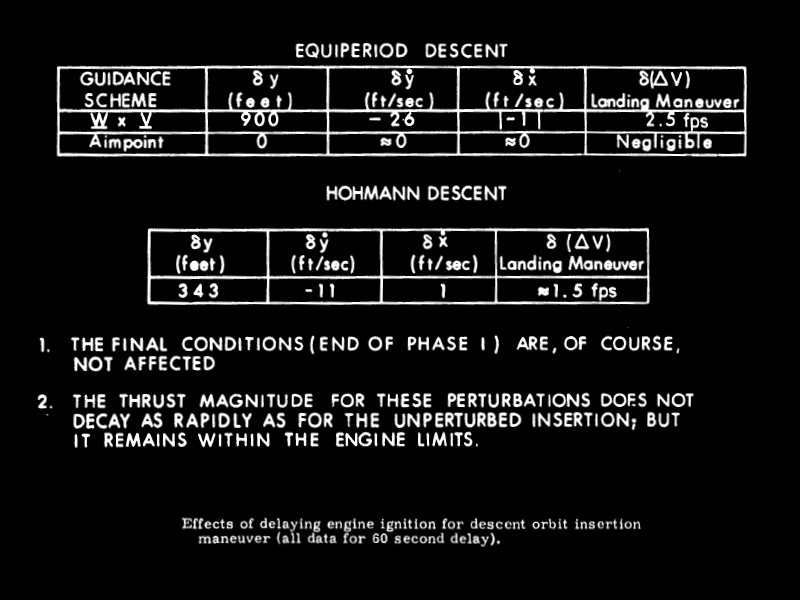Figure 14. Effect of delaying engine ignition.

Note that a delay of 60 seconds is tolerable. Thus the engine ignition window for the landing maneuver is an order of magnitude smaller than the engine ignition window for the descent orbit injection maneuver.

3 Landing Maneuvers from Hohmann Descents

The characteristics of a typical landing maneuver trajectory controlled by the E guidance equations of Section 2 are summarized in Figs. 15 through 23.

Figure 15. Landing maneuver from Hohmann orbit.

Figure 15 illustrates the altitude-range profile for the first two phases of the landing maneuver initiated from a Hohmann descent orbit.

Figure 16. Altitude vs. miles-to-go.

Figure 16 shows the plume 2 characteristics which were chosen such that acceptable visibility conditions were met. (Figures 4 and 5 show the thrust magnitude and angle for this trajectory.)

Figure 17. Altitude vs. time (sec.).

Figures 17 through 20 summarize the general landing maneuver position and velocity conditions as a function of time.

Figure 18. Range-to-go (x) vs. time (t) (sec.).

  

Figure 19. Speed vs. time (sec.).

Figure 20. Altitude rate (vertical speed) vs. time (sec.).

With reference to Fig. 20, it can be seen that the maximum vertical velocity condition is 180 ft/sec and occurs just prior to the second phase of the landing maneuver.

Figure 21. dV performance summary.

The dV requirements for the first two phases of the landing maneuver are summarized at the top of Fig. 21. The desired hover conditions at the end of phase 2 are an altitude of 200 feet with a velocity of 10 ft/sec along a -10° flight path angle relative to the local horizontal. The total dV requirement of 6048 ft/sec for these two phases controlled by the landing guidance equations is then compared with other types of landing maneuvers and conditions. If a "one piece" descent from engine ignition to hover is controlled by the landing guidance equations, a dV of 5805 ft/sec is required. This indicates that the two phase maneuver with its associated vehicle altitude and time constraints in phase 2 requires an additional 243 ft/sec dV requirement compared with the more optimum single phase maneuver in which all visibility would be sacrificed. The optimum dV trajectory listed in Fig. 21 was generated by a numerical steepest descent optimization program and required 10 ft/sec less total dV than the single phase E guidance case. This indicates that the E guidance concept described in chapter 2 is very close to optimum dV conditions for the landing maneuver.

Figure 22. Look angle vs. time (sec.).

The time history of the look angle during the second phase of the landing maneuver is shown in Fig. 22. The look angle, lambda, is defined as the angle between the line of sight to the landing site and the thrust or -x LEM vehicle axis. The minimum visibility limit of the present LEM window configuration is 25° as shown. The landing maneuver considered in this section resulted in a look angle of 32°. i.e., 7° above the lower edge of the LEM window. The visibility angle and landing site monitoring during phase 2 are described in detail in another section.

Figure 23. dV requirements for phase 2 constraints.

The dV penalty associated with various values of the minimum look angle. Lambda_MIN, during the second phase is summarized in Fig. 23. Approximately 100 ft/sec additional dV is required to increase the minimum visibility angle from 26° to 36° if the phase 2 maneuver time is held fixed at 115 seconds. With reference to Fig. 23, it can be seen that as the minimum look angle, lambda_MIN, is increased, the phase 2 initial altitude, vertical velocity, and range to go all decrease, thus lower thrust levels are commanded. These are desirable effects for astronaut monitoring, but require dV penalties that make them doubtful.

It should be noted that the landing maneuver characteristics presented in this section assumed a point mass LEM vehicle and no LEM attitude or throttle system dynamics were considered. The results of current guidance equation simulations which include the LEM vehicle dynamics will be presented in a future report.


[Chapter 4 (Performance Estimations) and chapter 5 (Equal Period Descents) have been skipped. See original paper /1/ if required.]

6 Hover and Touchdown Phase.

This final phase of the landing maneuver starts from the hover conditions established by the previous second or constant attitude phase of the maneuver. As described in chapter 2, the boundary conditions for the constant attitude phase are an altitude of 200 feet over the desired landing site with a velocity in the order of 10 ft/sec or less. The astronaut has the option of several modes of operation from these hover conditions. These modes of operation include a completely manual landing maneuver, a completely automatic landing maneuver controlled by the inertial units of the primary GN system, or some combination of manual and automatic modes to provide a semi-automatic or pilot assisted landing. The type of terminal letdown and landing maneuver will depend on the lunar surface conditions, and how they interact with the descent engine exhaust gases.

Under normal operation, the landing radar updating process is completed prior to the final letdown maneuver from the hover altitude. The automatic or semi-automatic modes of operation are then controlled from the inertial units of the primary GN system since landing radar data is questionable if severe dust or debris conditions occur because of interaction of the exhaust gases with the lunar terrain. The automatic mode of operation would involve a final landing radar update at the hover point with the visual check of the surrounding terrain and horizontal velocity conditions. This would be followed by a reduced throttle command which would build up a downward velocity followed by an increased throttle command to achieve a desired constant vertical velocity at a given altitude above the lunar terrain. This final constant velocity letdown would then be maintained by the inertial system until lunar contact had been made.

The semi-automatic mode of operation would be similar to the above automatic mode with the exception that the astronaut could interrupt this procedure at any point by an altitude hold mode of operation. When the astronaut selected this mode, the LGC would maintain control of the descent engine throttle servo and maintain a setting that would hold a constant altitude at the time of pilot control initiation. The astronaut would have complete control over the LEM attitude through the attitude controller and by pitching the vehicle in a desired direction he could effect translation maneuvers while the LGC maintained the constant altitude by thrust level control. When the astronaut has performed his desired translation maneuvers, the automatic system is reengaged, at which time any residual horizontal velocities are nulled and the automatic descent maneuver reestablished.

A hover altitude for the terminal conditions of the second landing maneuver phase were chosen arbitrarily, but are estimated to be the minimum altitude at which potential lunar dust problems would start (Ref. 2). The automatic let down maneuver from these hover conditions will require significant dV, depending upon various restrictions placed on the terminal letdown maneuver. The important parameters during the terminal letdown and their effects on the overall dV requirement are summarized in Fig. 56.

Figure 56. Lunar landing - hover to touchdown (automatic mode).

In this figure, the hover condition is assumed to be in an altitude of 200 feet with a zero velocity condition relative to the lunar surface. The first interval of the descent maneuver illustrated in the top of Fig. 56 requires reducing the descent engine throttle until a maximum vertical velocity V1 is achieved. The thrust is then increased so that the desired terminal descent velocity, V2, is established at some designated altitude, h2, after which the velocity V2 is maintained until surface contact is made. This operation can be illustrated by the first example of Fig. 56 in which the descent engine was throttled to its minimum setting for 5. 3 seconds until the maximum desired sink rate V1 of 15 ft/sec was achieved at an altitude of 160 feet, h1. The thrust of the descent engine was then increased over the next 9.5 seconds such that the desired terminal contact velocity V2 of 10 ft/sec was established by the time the vehicle reached an altitude h2 of 40 feet. This terminal velocity of 10 ft/sec was then maintained over the next 4 seconds until lunar surface touchdown was made. The total velocity requirement for this maneuver was 90.6 ft/sec as shown in Fig. 56. Fly comparing the various maneuvers Summarized in this figure with their associated maximum vertical velocities, V1; terminal contact velocities, V2; and altitude of the constant velocity phase h2; it can be seen that the dV requirements range between 70 and 130 ft/sec. The maneuvers summarized in Fig. 56 are near optimum type maneuvers for the various descent parameters considered. Actual maneuvers involving semi-automatic or pilot assisted landings will obviously require more dV than the near optimum descents summarized in this figure.

The primary reason that a hover altitude of 200 feet was chosen for the examples illustrated in this chapter for landing maneuvers was that the dV requirement increases for hover and terminal letdown maneuvers from higher altitudes. The effect of hover altitude on the dV requirement for the terminal maneuver is illustrated in Fig. 57.

Figure 57. Characteristic velocity vs. initial altitude for touchdown maneuver.

The curves illustrated in this figure are for the three velocity and altitude conditions previously considered in Fig. 56. These are the maximum allowed vertical velocity during the maneuver, V1; the desired terminal touchdown velocity, V2; and the altitude h2, at which the constant velocity must be established. It can be seen from Fig. 57, that all the conditions shown require essentially 100 ft/sec for automatic maneuver from 200 foot hover altitudes. As this hover altitude is increased to 1000 feet, the dV requirements range from approximately 300 to 500 ft/sec, depending upon the terminal descent maneuver characteristics chosen. As previously mentioned, the hover altitude will be chosen on knowledge of the lunar surface or dust conditions that are expected. The primary GN mode of operation up to the hover point condition requires that all final landing radar updating and astronaut visual monitoring be completed by the time the terminal letdown maneuver is initiated. The astronaut will still have the option of interrupted manual control, pilot assisted landing, if desired after this point.

At the present time. the descent engine cutoff criteria at the end of the terminal letdown has not been completely determined. The lunar surface, or dust conditions. and visibility limitations will be one of the major factors in determining what thrust termination criteria will be used. One of two approaches most often considered is to terminate thrust at an altitude of approximately 5 feet with zero velocity conditions. The uncertainty involved in this technique under heavy dust or no visibility conditions is that knowledge of altitude may not be available from the landing radar and errors would exist if extensive cratering was effected by the exhaust of the descent engine. An alternate approach would maintain the descent engine thrust until lunar contact had been made at the inertially controlled terminal velocity V2 of Fig. 56 at which time the thrust would be terminated. This technique would not depend on landing radar data and would be independent of cratering effects. The major problem with the latter technique is the dynamic effects on the LEM if one landing gear makes contact before the others under a throttle condition that essentially balances lunar gravity. The final engine termination criteria will depend on future simulations and knowledge of the lunar terrain.

An alternate method of third phase operation to touchdown is currently (1964) under investigation. This approach uses the same guidance concept as phase 2 to maintain visibility to the landing site as long as possible. The LEM does not came to a hover condition followed by a vertical descent in this approach, but the terminal conditions of phase 2 are chosen so that a near constant attitude can be maintained along a trajectory similar to that of phase 2 from altitudes of 200 feet to near surface contact. The results of this investigation are still preliminary and will be presented in a future report.

The primary GN system controls the LEM attitudes about the vehicle y and z axes throughout all automatically guided phases of the lunar landing maneuver. The vehicle orientation about the thrust axis (x axis) may or may not be controlled by the primary GN system during the first and third phases of the landing maneuver, but will be controlled during the second or constant attitude phase of the landing maneuver as described in another section. During the first phase of the landing maneuver, the vehicle z axis, may be directed downward so that the astronauts will be able to see the lunar surface until an altitude of approximately 30,000 feet is reached. At this time a 180° maneuver about the x axis is effected so that the window, or z axises in the up direction prior to the pitch-up on initial point of the second phase of the landing maneuver. It is important for primary GN operation that the attitude about the z axis be such that the windows are up when an altitude of 20,000 feet is reached, so that the landing radar can be used for updating altitude.

Figure 1.19. LEM landing radar antenna positions.

The current landing radar antenna Configuration is a two position arrangement such that the altitude measuring beam would be essentially vertical during the constant attitude phase (Fig l.19). This altitude beam could be used prior to the constant attitude phase at altitudes of approximately 20,000 feet. The second position of the landing radar antenna would be such that the altitude measuring beam would be vertical when the vehicle is in a vertical orientation at the hover conditions.

There is no primary GN system requirement for a preferred orientation of the LEM about the x axis at the time of lunar surface contact. The rendezvous radar gimbal axes have sufficient coverage to insure CSM tracking over the desired tracking sector (Section 5.3) under virtually any landing orientation. The three position AOT can achieve IMU alignments if the sun or earth are in the field of view for one fixed AOT position. The primary GN system places no restriction on the final touchdown orientation; however, if a choice is available it is preferred to direct the three positions of the AOT away from the sun or illuminated earth.

The primary GN System is maintained in the operating mode after lunar landing and descent engine cutoff for a period of time that is currently unspecified. This time interval is presently considered to be between 15 and 30 minutes in length, during which time the primary GN system can control an emergency take-off or abort if desired."



RESOURCES

/1/

•  (NASA CR-118610-Vol-1) PRIMARY G AND N SYSTEM LUNAR ORBIT OPERATIONS, VOLUME 1 (MIT) 258 p, R-446, edited by Norman E. Sears, April 1964
• This report was prepared under DSR Project 55—191, sponsored by the Manned Spacecraft Center of the National Aeronautics and Space Administration through Contract NAS 9—153.
• The following MIT Instrumentation Laboratory Apollo Space Guidance Analysis group personnel contributed to the preparation of this report:  D. S. Baker, R. D. Brown, G. W. Cherry, P. G. Felleman, R. D. Goss, E. S. Muller, R. J. Phaneuf, N.E. Sears (group leader), R. L. White, J. E. Young
• The publication of this report does not constitute approval by the National Aeronautics and Space Administration of the findings or the conclusions contained therein. It is published only for the exchange and stimulation of ideas.

/2/ Greek alphabet chart

Greek alphabet chart

* * *